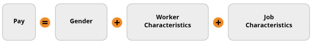
Measuring Pay Equity: Small Sample Size Individual Analysis
Individual-level analyses in pay equity investigations have two goals:
- identify individuals who may be negatively impacted by potential pay disparities,
- estimate the amount by which they may be negatively impacted.
When sample size is small and the 30/5-rule criteria cannot be met for regression analysis, individual-level analysis is still possible with data modeling approaches, but the results must be interpreted with caution and additional care.
There are many different methods to individual-level analysis. Here is a general analytical framework that can be applied to measure pay equity between individuals, including small sample size situations.
Overall, this approach involves two general steps:
- Step 1—Estimate Predicted Pay
- Step 2—Compute Individual Pay Difference
Please note that the method and steps detailed in this tool is not authoritative or definitive. The purpose of this tool is to provide a generic analytical framework that employers may use as a starting point and adapt and refined to the unique needs of their organization.
When sample size is small, it is not possible to complete a regression analysis among individuals performing substantially similar work to compute predicted pay. However, it is possible to compute an estimate of individual pay difference in standard deviation (SD) units, which is critical to identifying potentially underpaid individuals. The following provides an outline the steps to compute standardized pay difference:
Step 1: Estimate Quasi-Predicted Pay for Individual Employees
When sample size is small, quasi-predicted pay can be obtained from a regression analysis of company wide data. To estimate quasi-predicted pay for each employee, specify a regression model of worker and job characteristics but excludes any group indicator variables, (e.g., gender).
For example:
1. Regression Model for Pay Equity:
2. Regression Model for Pay Prediction:

It is important to note that quasi-predicted pay is not estimated from a group of individuals performing substantially similar work. Therefore, the absolute value of quasi-predicted pay does not directly indicate pay (in)equity. The relative value of quasi-predicted pay, however, is meaningful and will be used to compute individual standardized pay difference.
Step 2: Compute the Estimated Pay Differences for each Individual
Compute Raw Difference: After quasi-predicted pay is obtained for each individual employee, the next step is to compute the raw difference between actual-pay and quasi-predicted pay. These raw difference values are not relevant to pay equity analysis on their own, they must first be converted into standardized deviation units, as explained below.
Standardize Pay Differences by Substantially Similar Work Group: Once raw differences are computed, the next step is to identify and standardize the raw differences, separately, for each group who are performing substantially similar work. These standardize pay differences are interpretable and can be used to identify negatively impacted individuals.
Once raw differences are standardized by substantially similar work groups, it is possible to identify underpaid individuals even when the groups are small. Negative standardized pay differences indicate individuals who are underpaid.
Example:
A very simplified hypothetical example illustrates this process:
Step 1:
Regression model based on Company Wide Data: Quasi-Predicted Pay = 50,000Base Salary + 2,000 × Tenure + 10,000 × Performance
Step 2:
Compute Quasi-Predicted Pay Using Company Wide Data For the following hypothetical sample of employees with the given levels of Tenure and Performance, quasi-predicted pay is presented in the last column:
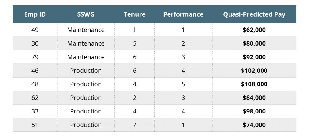
SSWG=Substantially Similar Work Group Please note, the absolute value of the quasi-predicted pay values should not be interpreted.
Step 3: Compute the Estimated Pay Differences for each Individual
The estimated raw pay difference for each employee is calculated as the difference between the employee’s actual pay and their predicted pay estimated in Step 1. For the hypothetical sample of employees:
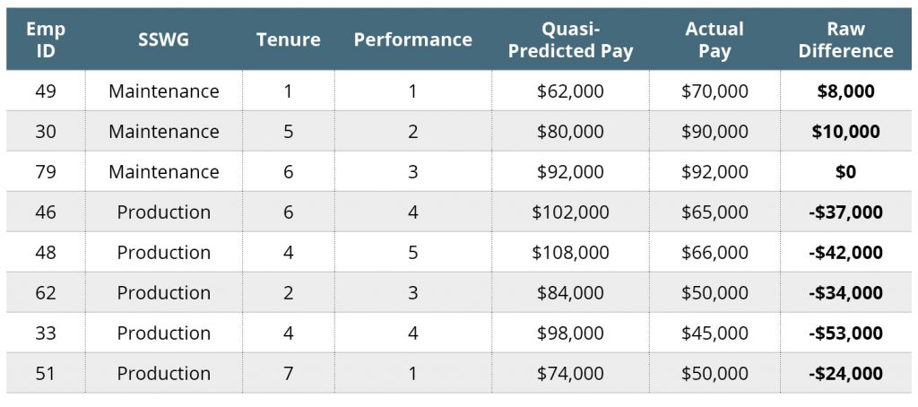
SSWG=Substantially Similar Work Group
Please note, the absolute value of the raw difference values should not be interpreted.
Step 4: Separately Standardized Raw Difference for Each Substantially Similar Working Groups
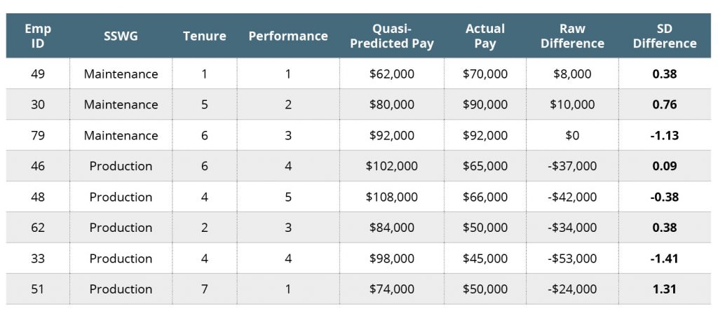
Separately standardize Raw Differences for each Substantially Similar Working Group (SSWG). In this example, standardized raw differences are computed for Maintenance employees and separately standardized raw differences are computed for Production employees. It is critical to compute standardized raw differences because the means and standard deviations for each SSWG are unique and different.
Interpreting SSWG=Maintenance: In this example, there are three individuals performing Maintenance work. It is important to only interpret the SD Difference results. Employees ID=49 and ID=30 have positive SD Differences—they are overpaid. Employee ID=79, however, is negative (SD=-1.13)—employee ID=79 is underpaid by 1.13 standard deviations.
Interpreting SSWG=Production. In this example, there are five individuals performing Production work. It is important to only interpret the SD Difference results. Employees ID=46, ID=51, and ID=62 have positive SD Differences—they are overpaid. The most overpaid is Employee ID=51—he is overpaid by 1.31 SDs. Employees ID=48 and ID=33 have negative SD differences. Employee ID=48 is -0.38 standard deviations below, and employee ID=33 is -1.41 standard deviations below.
The Production workers example demonstrates why interpreting Raw Differences can be misleading. In this case, all five production workers have negative raw differences, which may suggest that everyone is underpaid. These absolute differences are not meaningful because they are computed from quasi-predicted pay. By standardizing the raw differences, into SD Differences, it is possible to estimate the RELATIVE difference in pay between these five production employees. In this case, employee ID=46, ID=62, ID=51 are overpaid and employee ID=38 and ID=33 are underpaid.
Next Step
Once the individual pay gaps are computed and the underpaid individuals are identified, the next step is to investigate the cause of that gap. This is often referred to as a “cohort analysis.” See, cohort analysis for details on cohort analysis methods

DISCLAIMER: The materials provided on this web site are for informational purposes only and not for the purpose of providing legal advice. You should contact an attorney to obtain legal advice about any particular issue or problem. The materials do not represent the opinions or conclusions of individual members of the Task Force. The posting of these materials does not create requirements or mandates.